
The class "TVM4155 Numerical modelling and hydraulics" teaches the students basic theory of 1D, 2D and 3D numerical models used in water engineering. Homeworks include using HEC-RAS, SSIIM and OpenFOAM, solving the 1D and 2D St. Venands equations and the 3D Navier-Stokes equations. Also, sediment transport is included and the VOF method for computing free surface flow over spillways. Various processes in rivers and lakes/reservoirs are also explained, such as hydrodynamics, sediment transport, water quality, stratification and temperature. The lectures, assistance for homework and course material are given in English.
Prerequisite for taking the course: Previously having taken a course on basic fluid mechanics and hydraulics, for example TVM4116 Hydromechanics.
Lecturer: Nils Reidar B. Olsen
Lecture and homework plan for 2022
The course was taught on-line in 2021 and 2022 due to covid-19 restrictions. Lecture videos are given below.
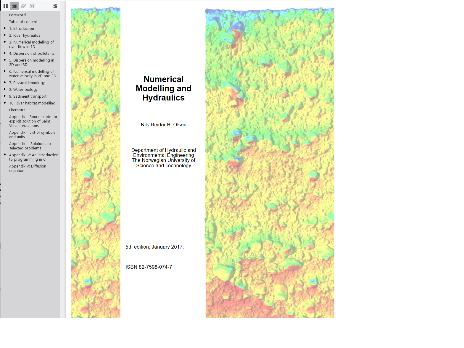
Class notes in English (1.6 MB PDF file) fom 2017.
There is assistance for the homework on campus every week.
Homework text
Additional information
Water surface profile problem text
Additional information
This homework was made by Peter Borsanyi.
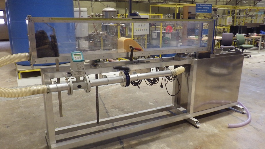
The laboratory measurements will be done in smaller groups. We will meet at VG2 and then go together to the laboratory.
Remember to bring a pen and paper, or some digital method to store the data you measure.
These files and other input files are found on the following web page.
The download web page for HEC-RAS is: http://www.hec.usace.army.mil/software/hec-ras/downloads.aspx
There are many instructional videos for HEC-RAS on YouTube. It is recommended that these are viewed first, to learn about the computer program. Search for "HEC-RAS Albrook", for example. There are also two videos about HEC-RAS in the Blackboard folder "Learning Material", where Per-Ludvig Bjerke talks about the program and the homework. Students who have an Apple Mac and no access to a Windows computer have two options:
1.Install the Wine program on the Apple Mac: https://www.winehq.org/ or http://winebottler.kronenberg.org/. Then install HEC-RAS and run it from your Apple Mac
2. You can borrow a Windows laptop from our department. The laptop must be signed for. You can not borrow it overnight. Therefore, you have to borrow the laptop at least one day before the homework starts, and install HEC-RAS 5.0.6 on it. And then borrow the same computer the morning of the homework.
The students must have installed HEC-RAS version 5.0.6 before the homework starts and they must also make sure that the program uses SI units. Additionally, the decimal sign "," must be set to "." (punktum). And it is an advantage to change the system area to USA and set the area format to English (USA) in "Setup for date, time and regiounal setup" ("Innstillinger for dato, klokkeslett og regionale innstillinger.")
PS! The students must NOT use the Norwegian letters "æøå" in the paths or file names used in this homework.
This homework was made by Kjartan Orvedal.
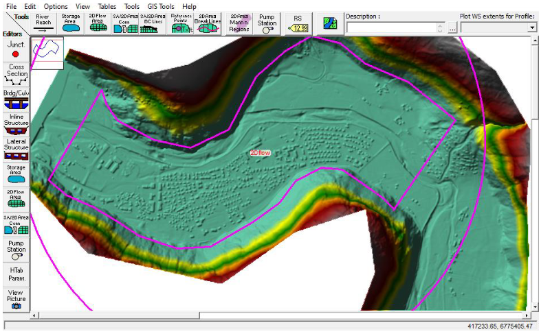
In this homework, the students will learn how to use the 2D version of HEC-RAS. The data is from the Lærdalselva in Western Norway. The attached PDF file gives instructions on what to do. The data needed is given in the .rar file. This file can be opened with tools given on the web page: https://www.winzip.com/win/en/lanrar.html
The instruction and input files are found on the following web page.
Instruction video on Panopto
This homework was made by Ana Juarez Gomez.
Use a spreadsheet to solve the problem. First, use a grid of 20x10 cells. Then increase the number of cells to 40x20. Use both first and second order upstream schemes for the computation. What are the results, and why do the results differ? What is the trap efficiency?
The implicit algorithms you have learned will give a circular reference in an Excel spreadsheet. To allow this in Excel for Windows, click File->Options->Formulas and click on "Enable iterative calculation". In Excel for Mac, click Excel menu, then Preferences->Calculations. Then "Use iterative calculation".
In LibreOffice Calc, click on Tools->Options->LibreOffice Calc->Calculate and click on Iterations in Iterative references.
Note that this video was recorded in 2021, so the dates/times mentionend in this video are not valid for this year.
This homework was made by Hans Bihs.
Note that this video was recorded in 2021, so the dates/times mentionend in this video are not valid for this year.
The homework on OpenFOAM is divided in two excersises, homework 9 and 10. This is the first part. Both parts are explained in the OpenFOAM videos, available under Learning Material.
Download of OpenFOAM should be done ahead of the guidance
Windows: http://www.cfdsupport.com/download-openfoam-for-windows.html
It is also possible to borrow a windows computer for the exercise, but you have to install the software at these computers as well.
Note: The installation of the windows version is very simple (similar to installing a regular program on windows). The installation on mac and linux are a bit more involved, and requires to type some commands in the command window. This means that if the mac/linux user gets scared of the instructions given at the links, it may be a good idea to borrow a windows computer for the exercises. Nevertheless, I will try to give some guidance on this in the lecture.
Homework 9 consist of 3 parts:
Running a tutorial
The steps to perform the different task are described in detail in the assignment text. The workload may seem a bit overwhelming, but as long as your get your OpenFOAM version up and running, it shouldn't be that time consuming.
Attachments: The zipped folder weirOverflow.zip contains the template to be used for the second part of this homework.
The Excel sheet, weir22data.xls, attached to this excersise is for the last part of homework 9. The numbers that are already there describes the parabola for a spillway geometry, but you need to make a text file in the format that is suited for SSIIM. However, you should use the geometry from the laboratory exercise. Note the units in the weir.txt used in SSIIM has to be in meters. You will need the newest version of SSIIM2, version 183, for this task. The pdf-file SSIIM_STL.pdf describes the disired input for SSIIM2.
Reporting: From part 1 deliver paraView images from different timesteps, enough to show an outline of how the water moves, part two hand in the surface elevation graph and the discharge calculations. For part 3 hand in the weir.txt file and a paraFoam view of the STL-file.
Video on Panopto with introduction to Command Windows/Terminals/Linux/OpenFOAM
The OpenFOAM homeworks were made by Mari Vold, Silje K. Almeland and Nils Solheim Smith.
- Create a mesh using an STL-file and snappyHexMesh
The steps to perform the different task are described in detail in the assignment text. Additionally, under Learning material you can find a video series titled OpenFOAM Videos featuring detailed description of the homework and how to work with OpenFOAM.
A very useful and brief information about Linux commands are given at: https://files.fosswire.com/2007/08/fwunixref.pdf
The zipped folder ofassignment2.zip contains the template to be used for this assignment. The stl-file weir.stl is a stl-file to be used for those who did not do the optional part of homework 9.
In problem 3, use an initial concentration of 0.008 for Ammonia and 0.0 for Nitrate, instead of the values given in the problem text.
Sediment concentrations
Tip: To find the velocity in the sediment transport formula, it is possible to use Mannings equation. The Manning-Strickler friction factor can be found from the diameter of the sediments, using formula 2.2.5 in the class notes.
Note: A sediment transport formula gives the value pr width of the channel. So it is necessary to find the width and multiply that with the result from the formula.
Tip: To find the equation for a line through a scatter of measured values, it is possible to use Excel or another spreadsheet. In Excel, plot the values in a figure using the "scatter" option. Then click on the scatter points in the figure with the left and then the right mouse button. From the pop-up menu, choose "Add trendline". Then choose a logarithmic equation. Afterwards, left and right click the line and from the pop-up menu choose "Format" and "options". Then click on the box with "Display equation in chart". This shows the formula.
This homework was made by Nils Rüther.
There will be a written exam for four hours.
Exam (PDF) from 2016, with solution.
Homework 6 2D Sedimentation tank
Compute the trap efficiencey of a sedimentation tank that is 100 meters long and 5 meters deep. The water velocity is 0.2 m/s. Particles are flowing in at the start of the tank in the upper 0.5 meters at a concentration of 0.1 kg/m3. The fall velocity of the particles is 1 cm/s. The Strickler value is 70.
Homework 7 SSIIM introduction
The enclosed text describes the homework: Using a CFD model to compute the water flow in a channel with an obstruction.
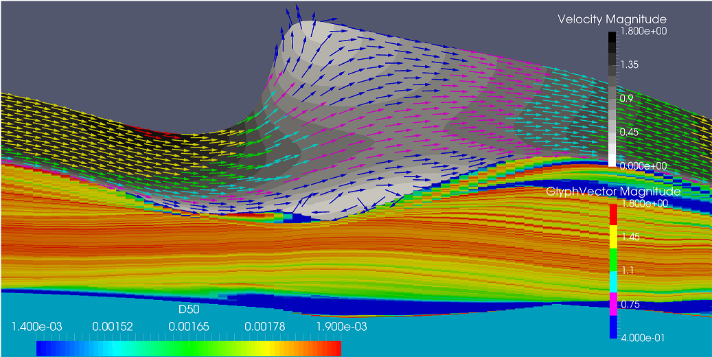
Homework 8 SSIIM desilting tank
The enclosed text describes the homework: Using a CFD model to compute the water and sediment flow in a sand trap/desilting basin.
Homework 9 OpenFOAM spillway 1
Linux/macOS: https://openfoam.org/download/
To get a feeling of the workflow
Running a spillway case where you do some changes to a given template
Get familiar with grid generation with blockMesh
Get familiar with some relevant post-processing tools in paraFoam
Create a STL-file to be used in the next exercise (optional)
Homework 10 OpenFOAM spillway 2
Homework 10 consist of 2 parts:
- Compare results from CFD with results obtained in the laboratory
Homework 11 Water quality
Do problem 2 and 3 in Chapter 8 of the class notes by using a spreadsheet. Compare the answer in problem 2 with the analytical formula. Assume kr = kd, and roc = 1.
Homework 12 Sediment transport
Compute the annual sediment discharge in a river using the enclosed annual hydrograph. Compute the sediment discharge both from the measured concentrations (enclosed) and from a sediment transport formula.
Water discharge
Exam
Exam (PDF) from 2017, with solution.
Exam (PDF) from 2018, with solution.
Exam (PDF) from 2019.
Exam (PDF) from 2021.
The web page is made by
Nils Reidar B. Olsen
|
Updated: 29. November 2025 |
|